13 Log-Normal Distribution – Data Science with R

13.1 Introduction

Some real-life variables can only take positive values and often show a strong right skew, meaning most values are clustered near the lower end, while a few are much higher. Examples include income, stock prices, the size of cities, and the number of views a video might get online. In these situations, the log-normal distribution often provides a better fit than the Normal distribution.

A variable follows a log-normal distribution if its logarithm is normally distributed. In other words, when we take the natural log of such a variable, the transformed values line up in the familiar bell-shaped curve of the Normal distribution. This happens because many of these processes are multiplicative in nature—growth occurs in ratios or percentages. Taking the logarithm converts these multiplicative effects into additive ones, and it is well known that sums of many small effects often follow a Normal distribution.

This makes the log-normal distribution a natural model for skewed, positive-valued data that arises from multiplicative processes.

13.2 When do we encounter the Log-Normal Distribution?

To understand when the log-normal distribution is appropriate, it helps to think about how quantities grow or change.

Some variables grow in additive steps. For example, if someone adds about $10 to their savings every week, the total increases by a respective amount each time. The distribution of total savings after a couple of years would then follow the normal distribution, since adding up many small effects tends to produce the bell-shaped curve.

But many real-world variables grow multiplicatively, meaning they change by a percentage or a ratio. Think of an investment that grows by 5% per year. The increase does not refer to a fixed dollar amount; it depends on how much is already saved. The same is true for bacterial populations, compound interest, and even social media followers, where a larger base can lead to faster growth. These are all examples where growth happens in terms of multipliers.

This is where logarithms come in. As discussed in Chapter Logarithms, the logarithm of a product turns multiplication into addition:

\[ log(X_1 \cdot X_2 \cdot X_3) = log(X_1) + log(X_2) + log(X_3) \]

So if a variable is shaped by the product of many small, independent effects, such as daily percent changes in a stock price, then its logarithm becomes the sum of many small effects. And as we’ve seen before, sums of many small effects tend to look normal. That means the original variable is log-normal.

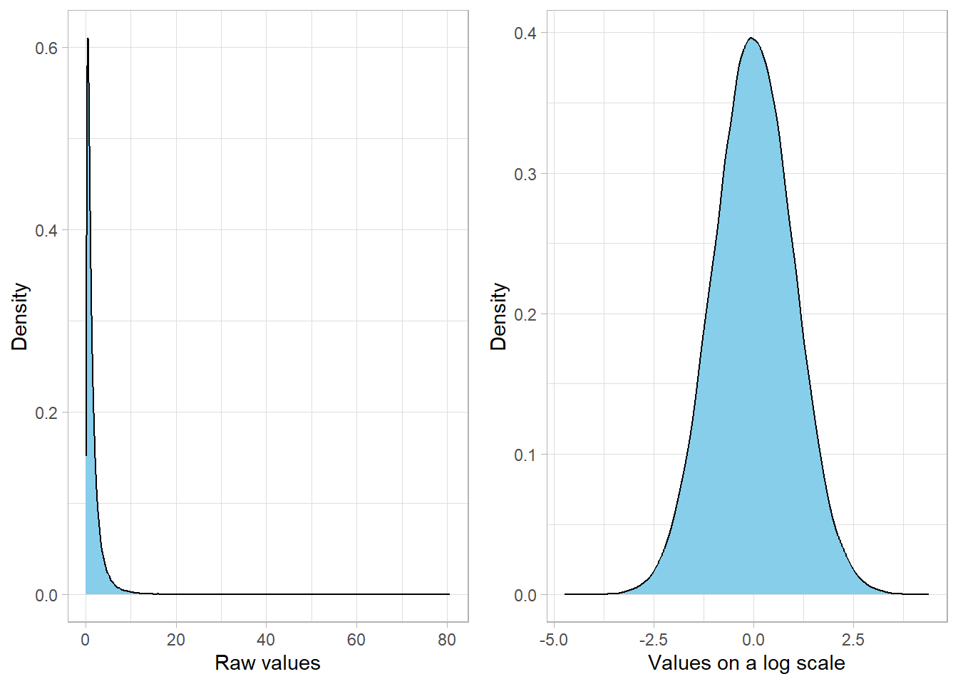
Let’s visualize this idea by simulating a variable that follows a log-normal distribution and comparing its shape to the shape of its logarithm:

It is apparent that the variable x is heavily skewed to the right on its original scale. But once we take the logarithm, the transformed values form a nice, symmetric bell-shaped curve.

Log transformation

The logarithm of a log-normal variable follows a normal distribution with mean $\mu$ and standard deviation $\sigma$. In our example, since we used $\mu = 0$ and $\sigma = 1$, the log-transformed values form a standard normal distribution centered at zero with unit spread.

A classic example of a multiplicative process is salary data, which we discussed in the Statistical Distributions chapter. Salaries rarely follow a Normal distribution. Instead, most people earn around a certain level, while a smaller group earns much higher incomes, creating a long right tail. This happens partly because income growth is often proportional rather than fixed—for example, raises are usually given as percentages, and promotions or bonuses build on past earnings. In addition, salaries are shaped by factors such as industry, education, and career progression, which interact in uneven ways. Together, these multiplicative and unequal effects make salary distributions skewed rather than symmetric—a pattern well described by the log-normal distribution.

13.2.1 What are the parameters and shape of the Log-Normal Distribution?

We write the log-normal distribution using the following notation:

\[ X \sim LogNormal(\mu, \sigma^2) \]

Here, $\mu$ is the mean of the natural logarithm of the variable, and $\sigma$ is the standard deviation of the natural logarithm of the variable. That is, the log-normal distribution describes a variable whose logarithm is normally distributed. In other words:

\[ log(X) \sim Normal(\mu, \sigma^2) \]

This property is what gives the log-normal distribution its name and behavior. It transforms a bell-shaped, symmetric distribution (normal) into a positively skewed one. The skew comes from the exponential transformation, which stretches out high values while compressing low ones.

The probability density function (PDF) of the log-normal distribution is:

\[ f(x) = \frac{1}{x\sigma\sqrt{2\pi}} exp(-\frac{(lnx - \mu)^2}{2\sigma^2}), x > 0 \]

This tells us the relative likelihood of observing a particular value of $x$. Because of the $\frac{1}{x}$ term, the density drops off quickly for small values, and because of the exponential, it has a long right tail for large values.

The expected value and variance of a log-normal variable are not μ and σ directly. Instead, we calculate these values using the following formulas:

\[ E(X) = e^{\mu + \frac{\sigma^2}{2}} \] \[Var(X) = (e^{\sigma^2} - 1) \cdot e^{2mu + \sigma^2}\]

These formulas might look a bit complex, but they make intuitive sense when we remember that the log-normal distribution stretches out values due to its exponential nature.

As an example, consider a variable that follows a log-normal distribution with $\mu = 0$ and $\sigma = 1$, which is the same distribution we visualized earlier. From the plot, we observed that the peak of the distribution occurs near $x = 0.5$, where the density is approximately 0.6. We can confirm this by evaluating the PDF at $x = 0.5$ using the formula:

\[ f(0.5) = \frac{1}{0.5 \cdot \sqrt{2\pi}} \cdot exp(-\frac{(ln0.5)^2}{2}) = \frac{1}{1.2533} \cdot 0.7864 \approx 0.6275 \]

Also, the expected value and the variance are the following:

\[ E(X) = e^{0 + \frac{1^2}{2}} \approx 1.65 \] \[Var(X) = (e^1 - 1) \cdot e^{0 + 1} \approx 4.67\] ## Calculating and Simulating in R

R provides built-in functions for working with the log-normal distribution, just like it does for the normal and other continuous distributions. These functions allow us to simulate data, compute densities, calculate cumulative probabilities, and find quantiles.

Let’s say we want to simulate how long it takes students to finish a test, where completion times are positively skewed and strictly positive, a situation where the log-normal distribution is appropriate. We can use rlnorm() to generate such data. For example, suppose the logarithm of test times follows a normal distribution with a mean of 3 and a standard deviation of 0.5. This means the actual times follow a log-normal distribution with the same parameters.

# Setting seed
set.seed(456)

# Simulate 2000 test times
lognorm_sim <- tibble(Time = rlnorm(2000, meanlog = 3, sdlog = 0.5))

# Plot the distribution
lognorm_sim %>%
  ggplot(aes(x = Time)) +
  geom_histogram(fill = "lightblue", bins = 30) +
  labs(x = "Test Time", 
       y = "Count")

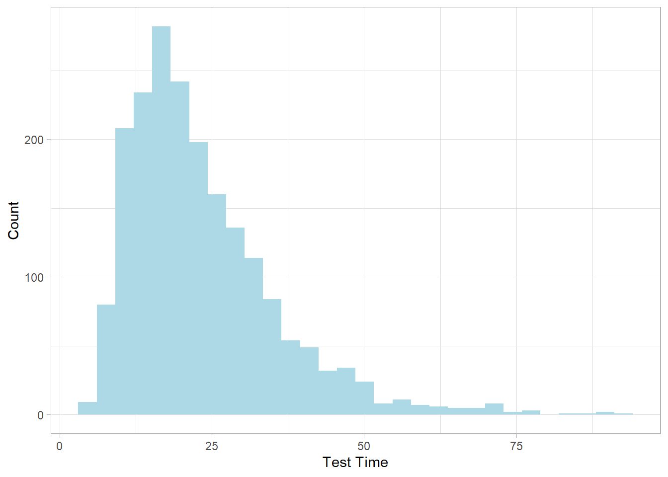
This histogram shows the characteristic right-skewed shape of the log-normal distribution: most students finish around the lower end of the range, but a few take much longer.

To calculate the probability density for a specific time, let’s say the likelihood that a student finishes in exactly 20 minutes, we use the dlnorm() function:

# Density at x = 20
dlnorm(x = 20, meanlog = 3, sdlog = 0.5)

[1] 0.03989277

To compute the probability that a student finishes in 20 minutes or less, we use the cumulative distribution function plnorm():

# Probability of finishing ≤ 20 minutes
plnorm(q = 20, meanlog = 3, sdlog = 0.5)

[1] 0.4965949

Conversely, if we want to know the time within which 75% of students are expected to finish, we can use the quantile function qlnorm():

# 75th percentile
qlnorm(p = 0.75, meanlog = 3, sdlog = 0.5)

[1] 28.14149

These functions make it easy to simulate, explore, and interpret data that follows a log-normal pattern. Whether you’re modeling completion times, reaction speeds, income levels, or biological growth, the tools in R allow you to connect the theoretical properties of the distribution to practical questions and real-world data.

13.3 Recap

The log-normal distribution is a useful model for continuous variables that are strictly positive and right-skewed. It is defined by two parameters: the mean and standard deviation of the logarithm of the variable. Simply put, if the logarithm of a variable is normally distributed, then the variable itself follows a log-normal distribution.

What sets the log-normal distribution apart is its natural fit for variables that grow or change multiplicatively—that is, in terms of percentages or ratios rather than fixed amounts. It is this multiplicative behavior creates a long right tail, with most values clustered near the lower end and a few very large values.

Because the log-normal arises from the exponential of a normal variable, its mean and variance are larger than the mean and standard deviation of the logged values. This reflects how multiplication of many small factors compounds variability.